Source/Sink & External Fluxes
Source/Sink loads and External Fluxes are optional entries defined in the Master configuration under OPENWQ_INPUT.
They use a similar data structure. The differences are highlighted in each section below.
Each sink/source or external flux is defined in an individual JSON file, and you can add as many files as desired.
There are five ways to provide source/sink data:
JSON – inline time series in the JSON file
CSV/ASCII – time series in an external CSV file
Copernicus LULC (static coefficients) – land-use-based loading using Copernicus satellite data and static export coefficients
Copernicus LULC (dynamic coefficients) – extends Method 3 with precipitation and temperature scaling (SWAT-inspired)
ML Model – XGBoost or Random Forest trained on monitoring data (EPA XGBest-inspired)
Common Structure
All source/sink and external flux JSON files share the following top-level structure.
Key 1: METADATA
|
Comments or relevant information about the data |
|
Additional information or additional comments |
Key 2: (i#) (numbered entries in sequential order)
Each numbered entry defines one loading or flux:
Method 1: JSON (inline data)
Set DATA_FORMAT to "JSON". The DATA block contains the time series directly in the JSON file.
Each entry is a numbered row with the format:
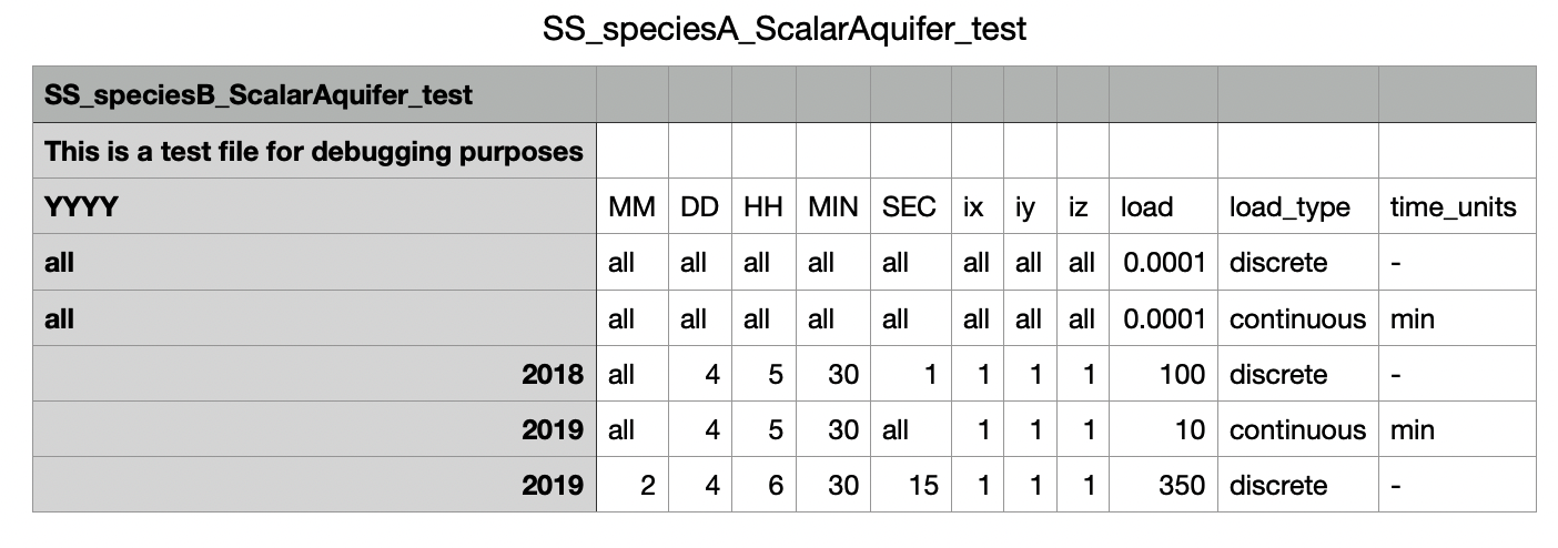
"(i#)": [YYYY, MM, DD, HH, MIN, SEC, ix, iy, iz, load, load_type, time_units]
Using Host Model Cell IDs (cell_id mapping)
Instead of using internal OpenWQ indices (ix, iy, iz), you can specify the cell identifier from the host model directly in the <ix> field. OpenWQ will automatically look up the corresponding (ix, iy, iz) indices using the cellid_to_wq mapping provided by the host model coupler.
The cell_id is a single string that uniquely identifies a spatial element across all dimensions (ix, iy, iz). The exact format depends on how the host model coupler populates the mapping:
mizuroute: Uses reach IDs directly (e.g.,
"1200014181")SUMMA: Combines HRU ID with layer index (e.g.,
"123456_z1","123456_z2")
When OpenWQ encounters a string value in the <ix> position that is not "all", it searches the cellid_to_wq mapping to find the corresponding internal indices. If found, the <iy> and <iz> values in the JSON are ignored since the cell_id uniquely identifies all three dimensions.
Example for mizuroute (1D river network):
"DATA": {
    "1": [2018, 6, 15, 0, 0, 0, "1200014181", 1, 1, 1000, "discrete"]
}
Example for SUMMA (multi-layer soil):
"DATA": {
    "1": [2018, 6, 15, 0, 0, 0, "123456_z1", 1, 1, 500, "discrete"],
    "2": [2018, 6, 15, 0, 0, 0, "123456_z2", 1, 1, 300, "discrete"]
}
This feature:
Eliminates the need to know internal OpenWQ index mappings
Uses the same identifiers visible in the HDF5 output files (printed under the
cellid_to_wqlabelcolumn, e.g.,reachId,hruId)Works globally for all host model couplings that provide the
cellid_to_wqmappingFalls back to standard index parsing if the cell_id is not found (with a warning message)
Note
Check the HDF5 output files to see the exact cell_id format used by your host model. The cell IDs are printed in the output alongside the water quality results, making it easy to identify which identifier to use in your input files.
Example:
{
    "METADATA": {
        "Comment": "synthetic loading",
        "Source": "test_1"
    },
    "1": {
        "CHEMICAL_NAME": "species_A",
        "COMPARTMENT_NAME": "SCALARAQUIFER",
        "TYPE": "source",
        "UNITS": "kg",
        "DATA_FORMAT": "JSON",
        "DATA": {
            "1": ["all","all","all","all","all","all","all","all","all",0.0001,"discrete"],
            "2": ["all","all","all","all","all","all","all","all","all",0.0001,"continuous","min"],
            "3": [2018,"all",4,6,30,30,1,1,1,100,"discrete"],
            "4": [2019,"all",4,6,30,"all",1,1,1,10,"continuous","min"],
            "5": [2019,2,4,6,30,15,1,1,1,350,"discrete"]
        }
    }
}
Example using cell_id (mizuroute reach_id):
{
    "METADATA": {
        "Comment": "N loading from fertilizer using reach IDs",
        "Source": "fertilizer_application"
    },
    "1": {
        "CHEMICAL_NAME": "NO3-N",
        "COMPARTMENT_NAME": "RIVER_NETWORK_REACHES",
        "TYPE": "source",
        "UNITS": "kg",
        "DATA_FORMAT": "JSON",
        "DATA": {
            "1": [2018, 6, 1, 0, 0, 0, "1200014181", 1, 1, 500, "discrete"],
            "2": [2018, 6, 15, 0, 0, 0, "200014182", 1, 1, 300, "discrete"],
            "3": [2018, 7, 1, 0, 0, 0, "1200014181", 1, 1, 250, "discrete"]
        }
    }
}
Example using cell_id (SUMMA hruId with layer):
{
    "METADATA": {
        "Comment": "Fertilizer loading to soil layers",
        "Source": "agricultural_input"
    },
    "1": {
        "CHEMICAL_NAME": "NO3-N",
        "COMPARTMENT_NAME": "ILAYERVOLFRACWAT_SOIL",
        "TYPE": "source",
        "UNITS": "kg",
        "DATA_FORMAT": "JSON",
        "DATA": {
            "1": [2018, 6, 1, 0, 0, 0, "12345_z1", 1, 1, 500, "discrete"],
            "2": [2018, 6, 1, 0, 0, 0, "12345_z2", 1, 1, 300, "discrete"],
            "3": [2018, 6, 1, 0, 0, 0, "67890_z1", 1, 1, 400, "discrete"]
        }
    }
}
Method 2: CSV/ASCII (external file)
Set DATA_FORMAT to "ASCII". The time series is provided through an external CSV file.
The DATA block points to the file instead of containing inline data.
|
Path to the CSV/ASCII file with the input data |
|
Delimiter used in the file, e.g., |
The header row is auto-detected: the C++ parser scans each line for the YYYY column name.
Everything before the header is ignored; everything after it is treated as data.
Required columns: YYYY, MM, DD, HH, MIN, SEC, ix, iy, iz, load, load_type, time_units
Example:
{
    "METADATA": {
        "Comment": "CSV-based loading",
        "Source": "fertilizer_data"
    },
    "1": {
        "CHEMICAL_NAME": "species_B",
        "COMPARTMENT_NAME": "SCALARAQUIFER",
        "TYPE": "source",
        "UNITS": "kg",
        "DATA_FORMAT": "ASCII",
        "DATA": {
            "FILEPATH": "SS_speciesA_ScalarAquifer_test.csv",
            "DELIMITER": ","
        }
    }
}
Method 3: Copernicus LULC with static coefficients
The Python configuration generator can compute spatially distributed source/sink loads based on Copernicus ESA CCI Land Use/Land Cover (LULC) satellite data. This method:
Reads Copernicus LULC NetCDF files (
ESACCI-LC-*.nc)Clips the raster data to the catchment boundary using a shapefile
Computes the area of each land use class per HRU (Hydrological Response Unit)
Generates per-HRU, per-year loading CSV files
Creates the OpenWQ source/sink JSON configuration referencing those CSV files
This is configured in the Python model_config_template.py using:
ss_method = "using_copernicus_lulc_with_static_coeff"

# Basin shapefile information
ss_method_copernicus_basin_info = {
    "path_to_shp": "path/to/catchment.shp",
    "mapping_key": "HRU_ID"
}

# Directory containing Copernicus LULC NetCDF files
ss_method_copernicus_nc_lc_dir = "path/to/copernicus_lulc/"

# Period to process [year_start, year_end]
ss_method_copernicus_period = [2000, 2020]

# Compartment name for the loads
ss_method_copernicus_compartment_name_for_load = "SUMMA_RUNOFF"
The generator creates a ss_copernicus_files/ subdirectory containing the clipped rasters, per-HRU area tables, and the resulting CSV loading files that are referenced by the generated JSON configuration.
Method 4: Copernicus LULC with dynamic coefficients
This method extends Method 3 (Copernicus LULC with static coefficients) by applying monthly precipitation and temperature scaling to the annual export coefficients. It distributes annual loads across months using a combined hydrological-biological weight, inspired by SWAT’s precipitation-driven loading and Q10 temperature scaling.
Monthly weight formula:
where:
\(P_m\) is monthly precipitation (mm)
\(\alpha\) is the precipitation scaling power (default 1.0; higher values amplify runoff sensitivity)
\(Q_{10}\) is the biological rate doubling per 10 C (default 2.0)
\(T_m\) is monthly temperature (C)
\(T_{ref}\) is the reference temperature (default 15 C)
Weights are normalized so that monthly loads sum to the annual load for each nutrient and HRU.
This is configured in the Python model_config_template.py using:
ss_method = "using_copernicus_lulc_with_dynamic_coeff"

# Climate data: monthly precipitation (mm) and temperature (C) per year
ss_climate_data = {
    2018: {
        "precip_mm": [80, 60, 70, 90, 110, 80, 50, 45, 65, 85, 95, 100],
        "temp_c": [-5, -3, 2, 8, 14, 19, 22, 21, 16, 10, 3, -2]
    },
    2019: {
        "precip_mm": [75, 65, 80, 95, 100, 75, 55, 50, 70, 80, 90, 85],
        "temp_c": [-4, -2, 3, 9, 15, 20, 23, 22, 17, 11, 4, -1]
    }
}

# Precipitation scaling power (default 1.0)
ss_climate_precip_scaling_power = 1.0

# Q10 temperature scaling (default 2.0; biological rate doubling per 10C)
ss_climate_temp_q10 = 2.0

# Reference temperature (C) for Q10 scaling
ss_climate_temp_reference_c = 15.0
The method reuses the Copernicus LULC pipeline for spatial area computation, then applies the climate adjustment to redistribute the annual loads across months. The output is standard JSON DATA_FORMAT entries that the C++ runtime processes transparently.
Note
This method requires the same Copernicus LULC configuration parameters as Method 3 (basin shapefile, LULC NetCDF directory, period, compartment name, and HDF5 mapping file).
Method 5: ML Model (XGBoost / Random Forest)
This method trains a machine learning model on water quality monitoring data and generates source/sink predictions. It is inspired by the EPA XGBest methodology, which demonstrated that tree-based models outperform traditional statistical methods (LOADEST, WRTDS) for daily nutrient load prediction.
Workflow:
Reads a monitoring CSV file containing dates, features (discharge, precipitation, temperature, etc.), and target nutrient concentrations
Engineers temporal features (month, day-of-year, cyclical sin/cos encoding)
Trains an XGBoost or Random Forest model per target species
Converts predicted concentrations to loads using discharge (if available)
Aggregates predictions to monthly time steps
Generates standard OpenWQ SS JSON with
DATA_FORMAT: "JSON"entriesSaves trained models in XGBoost text format (FastForest-compatible for future C++ runtime inference)
This is configured in the Python model_config_template.py using:
ss_method = "ml_model"

# Path to monitoring data CSV
# Must contain: 'date' column, feature columns, and target nutrient columns
ss_ml_training_data_csv = "path/to/monitoring_data.csv"

# Model type: "xgboost" or "random_forest"
ss_ml_model_type = "xgboost"

# Target species (nutrient column names in CSV)
# If None, auto-detected from non-feature numeric columns
ss_ml_target_species = ["NO3-N", "TP"]

# Feature columns (if None, auto-detected)
ss_ml_feature_columns = None

# Number of trees and max depth
ss_ml_n_estimators = 200
ss_ml_max_depth = 6
Expected CSV format:
date,discharge_m3s,precip_mm,temp_c,NO3-N,TP
2018-01-01,15.2,3.5,-2.1,2.3,0.05
2018-01-02,14.8,0.0,-3.0,2.1,0.04
...
Model outputs:
The script saves the following in ss_ml_model_files/:
ml_model_<species>.txt– XGBoost text dump (FastForest-compatible for C++ deployment)ml_model_<species>.json– XGBoost binary model (for Python reuse)ml_model_features.json– Feature configuration, metrics (R2, RMSE, MAE)
The generated SS JSON uses standard DATA_FORMAT: "JSON" entries, so no C++ runtime changes are needed. The existing CheckApply_EWFandSS_jsonAscii function processes the ML-predicted loads transparently.
Note
Dependencies: This method requires scikit-learn and xgboost Python packages. Install with: pip install scikit-learn xgboost
Note
Future C++ runtime inference: The trained XGBoost models are saved in text format compatible with the FastForest C++ library (header-only, no dependencies, thread-safe, C++98 compatible). This enables future integration for dynamic runtime inference based on live host-model state variables instead of pre-computed predictions.
HDF5 External Fluxes (inter-model coupling)
This method is only applicable to External Fluxes (not Sink/Source).
It is used when loading external flux concentrations from the HDF5 output of another host_model-OpenWQ coupled simulation (e.g., an atmospheric model providing precipitation chemistry to a hydrological model).
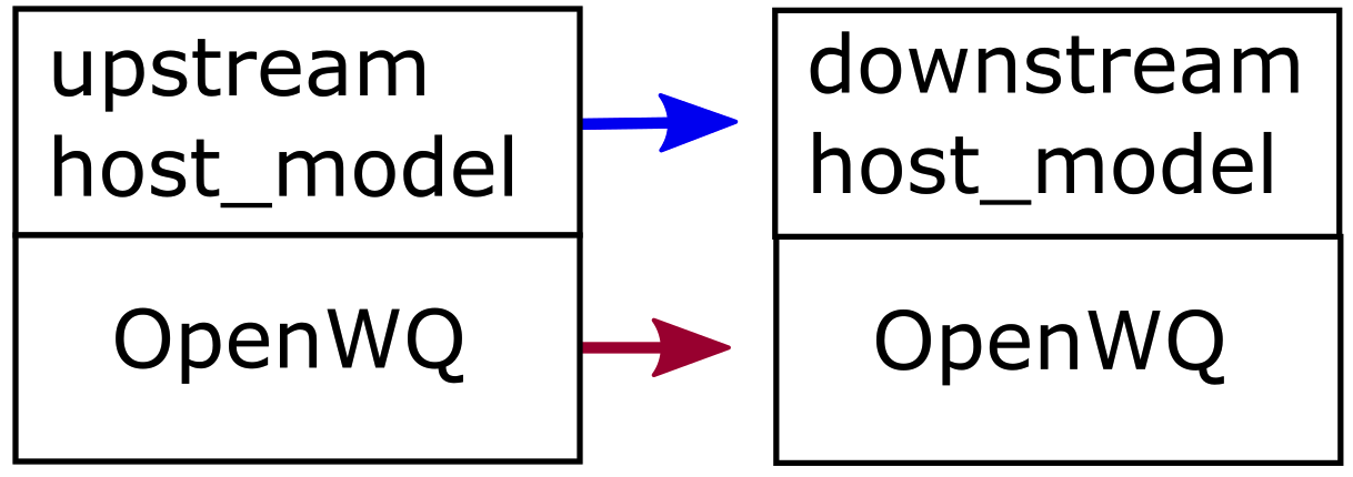
The general steps are:
Run the upstream host_model-OpenWQ coupled model. Export data for the compartment from where the inter-model fluxes originate.
Run the downstream host_model-OpenWQ coupled model, pointing to the upstream HDF5 outputs.
Additional keys for HDF5 external fluxes:
|
Name of the compartment in the upstream model from where the fluxes originate |
|
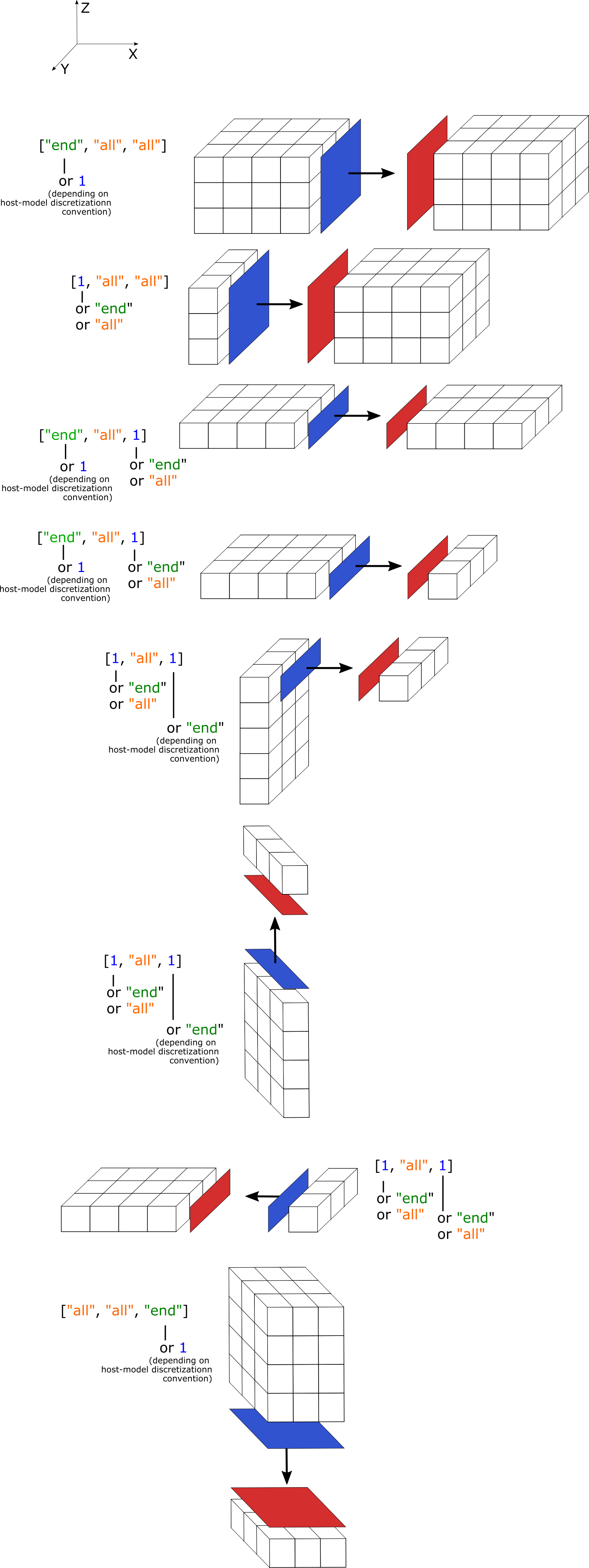
Array specifying the interface elements, e.g., |
|
Time interpolation method: |
|
Path to the HDF5 output folder from the upstream model
(must also contain |
Diagrams showing examples of "INTERACTION_INTERFACE" setup:
Example:
{
    "METADATA": {
        "Comment": "atmospheric deposition",
        "Source": "upstream_model"
    },
    "1": {
        "DATA_FORMAT": "HDF5",
        "UNITS": "mg/l",
        "EXTERNAL_COMPARTMENT_NAME": "ATMOSPHERE_LAYER",
        "EXTERNAL_INPUTFLUX_NAME": "PRECIP",
        "INTERACTION_INTERFACE": ["all", 1, 1],
        "INTERPOLATION": "LINEAR",
        "FOLDERPATH": "openwq_ewf_h5"
    }
}
The JSON file supports C/C++ syntax for comments: single-line comment (//) or comment blocks (/* and */).
The symbol (i#) refers to an integer number sequence. The symbol (s#) refers to a string input. The symbol (f#) refers to a float input value.